A recent arXiv post ignited an interesting discussion with students and colleagues, demonstrating once more how the Heisenberg picture in quantum mechanics can easily be misunderstood to the point of becoming almost paradoxical. Here I intend to briefly summarize what I think may be the crux of the problem (or problems). The argument below follows a discussion on the topic that I had with Masanao Ozawa few years ago; however, any error or misunderstanding in it is to be entirely attributed to me.

One-step evolutions

Suppose that we are following the evolution of a quantum system from an initial time to a later time , and that the unitary operator evolving the state of the system is , so that

.

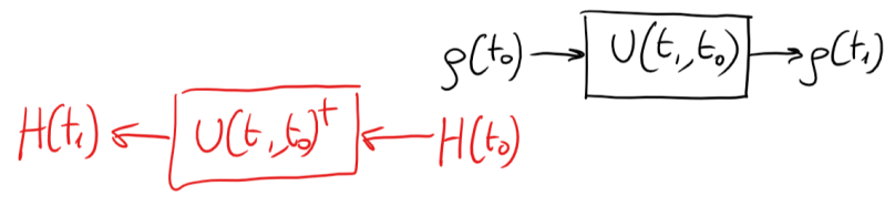
The latter is called the Schrödinger picture of the evolution. In this picture, states evolve in time, while observables (like the Hamiltonian) do not.

The Heisenberg picture is meant to do the opposite: it keeps states “freezed”, while observables evolve. It can be also understood as a “pullback” operation: very much like when one looks at a rotation from the viewpoint of vectors (Schrödinger picture) or the viewpoint of the coordinate system (Heisenberg picture).

For the two pictures to give consistent predictions, that is, , it is prescribed that, if an observable at time is denoted as , the same observable at the later time will be . From this relation, we see that the state evolves according to , while the observable evolves according to .

 

It is quite tempting at this point to interpret this by saying that “states evolve forward in time, while observables evolve backwards in time”. If only two times are considered, that seems just a curious though innocuous way of phrasing it. Indeed I have heard a lot of researchers explaining the Heisenberg picture this way. I myself would have nodded my head hearing this some years ago. However, I now see why this interpretation can be in fact very confusing, potentially leading to wrong calculations, when more than two times are considered.

Two-step evolutions: the wrong approach

Imagine now to fix three instants in times, and two unitary operators:  one, , describing the evolution of states from to as before; and another one, , propagating states from to . The problem is: how should one model the evolution of an observable from to ? A naive guess based on the “backwards-in-time evolution” intuition would suggest a scheme like the following:

But what should be the evolution operator describing the box denoted by question marks? As the arXiv post mentioned at the beginning of this post argues, one could be tempted to say that the right evolution operator is , probably by symmetry with the Schrödinger’s branch evolving forward in time. This naive guess leads to the equation .

Problem is, this is of course wrong! The correct thing to do is to understand that the total evolution of the state from to is given by the unitary operator . Consequently, one has that

.

This is the correct description of in the Heisenberg picture.

Another, more subtle, source of confusion

We have seen how the naive “backwards in time” interpretation is wrong. However, at this point, another structure emerges that still suggests some kind of “time-reversal”. I am speaking now of the fact that, in the correct equation, that is, , the order of the propagators is reversed with respect to the one that is used for states, that is .

Given that the equation itself is correct, in what follows I am simply criticizing its interpretation. I would like to argue, in particular, that, even though the evolution operators act in reverse order on the observable, the Heisenberg picture should not (or, at least, need not) be interpreted or explained as “backwards in time” evolution.

The point is that , on its own, has no meaning in the Heisenberg picture. In the Heisenberg picture, all operators must be evolved consistently. In particular, the operator , which is defined formally at , when applied at time , must also be consistently evolved before being applied on anything. (Better said, the Hamiltonian generating the unitary evolves in time and, with it, the unitary operator it generates.)

Hence, in the Heisenberg picture, the propagator of observables from to is not but its evolved version, that is,

.

If we substitute this into the initial formula, then we indeed obtain that , as it was computed at point 2 above.

However, once written as above, it gives us a very clear understanding of what is going on in the Heisenberg picture.

Summarizing, the Heisenberg picture is indeed a pullback transformation, but a pullback that happens forward in time. After all, both Heisenberg and Schrödinger pictures provide equivalent representations of exactly the same process, which of course happens forward in time.