…alias observational entropy!

In his 1932 book, von Neumann famously discusses a thermodynamic device, similar to Szilard’s engine, through which he is able to compute the entropy of a quantum state, obtaining the formula . I discussed about this in another post.

Probably less people know however that, just a few pages after having derived his eponymous formula, von Neumann writes:

Although our entropy expression, as we saw, is completely analogous to the classical entropy, it is still surprising that it is invariant in the normal (note added, in the sense of “unitary/Hamiltonian”) evolution in time of the system, and only increases with measurements — in the classical theory (where the measurements in general played no role) it increased as a rule even with the ordinary mechanical evolution in time of the system. It is therefore necessary to clear up this apparently paradoxical situation.

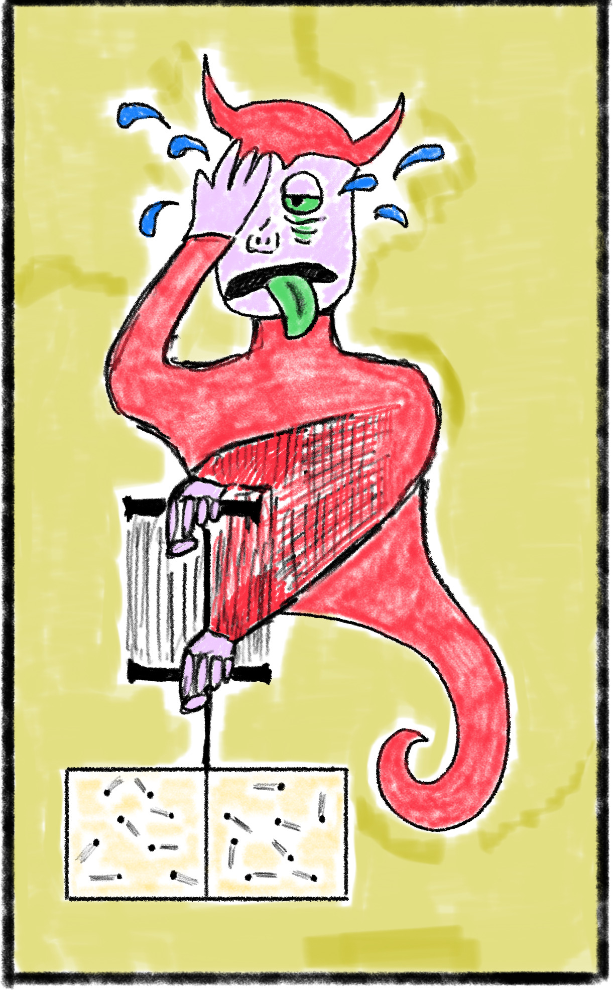
What von Neumann is referring to in the above passage is the phenomenon of free or “Joule” expansion, in which a gas, initially contained in a small volume is allowed to expand against the vacuum, thereby doing no work, but causing a net increase in the entropy of the universe, even though its evolution is Hamiltonian, i.e., reversible, all along.

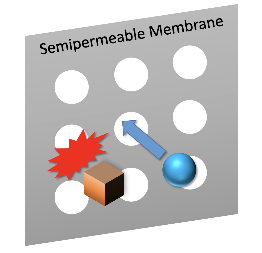
In order to resolve this issue, von Neumann suggests that the correct quantity to consider in thermodynamic situations is not (what we call it today) von Neumann entropy, but another quantity, that he calls macroscopic entropy (and which today is called observational entropy):

where denotes a fixed measurement, i.e., a POVM , is the expected probability of occurrence of each outcome, and are “volume” terms. The measurement, with respect to which the above quantity is computed, is used by von Neumann to represent, in a mathematically manageable way, a macroscopic observer “looking at” the system: the system’s state is , but the observer only possesses some coarse-grained information about it, and the amount of such coarse-grained information is measured by the macroscopic entropy.

In a paper written in collaboration with Dom Safranek and Joe Schindler and recently published on the New Journal of Physics, we delve into the mathematical properties and operational meaning of observational/macroscopic entropy, and discover some deep connections with the theory of approximate recovery and statistical retrodiction, which is a topic that keeps showing up in my recent works, even if I’m not looking for it from the start.

Is it perhaps because retrodiction really does play a central role in science? Or is it just me seeing retrodictive reasoning everywhere?

Arthur Eddington once famously wrote: “If your theory is found to be against the second law of thermodynamics, […] there is nothing for it but to collapse in deepest humiliation.” So why not take the second law as an axiom, on which physical theories are built, rather than as a consequence to be tested? The problem is that, in its conventional thermodynamic formulation, the second law relies on quite a lot of physics to have been already introduced, and it is not clear how one could assume its validity before other concepts like “work” or “heat” are even defined.

In a paper published today on Physical Review Research, we identify in von Neumann’s information engine the conceptual device that allows us to discuss the second law already from the early stages of the construction of a physical theory, when its most fundamental logical structures are being laid down. What we find is that, by concatenating two information engines in a closed cycle, the second law can be thought of as the requirement that no information can be created from nothing, thus guaranteeing the internal logical consistency of the theory.

From the popular summary of my paper with Arshag and Mark, “Thermodynamic constraints on quantum information gain and error correction” just published on PRX Quantum.

It is now widely accepted that Maxwell’s demon does not, in fact, break the second law of thermodynamics, if the energetic cost of resetting its memory is taken into account. This resolution of the paradox is known as Landauer’s principle.

In this work, we delve into the inner workings of Maxwell’s demon by considering how it behaves in the quantum error correction setting. We show that Landauer’s principle is only the limiting case of a more general triple trade-off relation between the thermodynamic, information-theoretic, and logic performances of the demon. For example, we show that for most measurements that the demon can perform, extracting work above the Carnot limit is penalized by a drop in the error correction fidelity. Moreover, when the demon successfully performs perfect error correction, work extraction above the Carnot limit becomes impossible with most quantum measurements. Finally, we realize that the amount of information that the demon can extract about the error type is bounded from above by the dissipated heat during that process. Interestingly, this also gives physical meaning to negative values of this information gain.

This #AVSQuantumScience paper shares a new approach to statistical mechanics that replaces reverse processes with consistent inference, clarifying the 2nd Law’s meaning and revealing new possibilities, classical and quantum alike. @quantumlah @AVS_Members https://t.co/ziG6JjmHAJ

— AIP Publishing (@AIP_Publishing) November 20, 2021

Position title and duration: postdoc or research assistant professor, depending on the candidate’s qualifications. The appointment is offered initially for a one-year period, with the possibility of further extensions up to three years of total duration.

Description: this position is offered by the Quantum Information Theory Group within the collaboration “Extreme Universe”, headed by Prof. Tadashi Takayanagi (YITP, Kyoto University). This collaboration brings together Japan-based world-renowned researchers in quantum information theory, quantum gravity, cosmology, and condensed matter physics, with the aim of creating new and exciting bridges between these very active areas of research. The successful candidate will work in close contact with Prof. Francesco Buscemi (Nagoya University), but is expected to interact also with the rest of the collaboration group and to participate in various interdisciplinary meetings within the project. The successful candidate is expected to commence their appointment on April 2022 or as soon as possible after that.

Requirements: applicants are expected to hold a PhD degree in a theoretical field related to quantum information sciences by the time they begin their appointment. Ideally, they will be familiar with recent ideas and techniques in quantum information theory and have at the same time strong interests in fundamental questions in theoretical physics.

Submission procedure: interested candidates should provide

1. a cover letter;
2. an up-to-date curriculum vitae;
3. a research statement;
4. an up-to-date list of research achievements (including published papers, preprints, talks, posters, etc.);
5. contact information of three references able to provide recommendation letters upon request.

The application can be done by sending the above documents directly to buscemi@nagoya-u.jp or through the project’s webpage at https://academicjobsonline.org/ajo/jobs/19880 (where also other openings are advertised)

Submission deadline: 30 November 2021

For further inquiries, please contact me at buscemi@nagoya-u.jp

Is there an observer-independent time-reversal in physics? Only for Hamiltonian dynamics, we argue. Otherwise there’s only retrodiction, which of course depends on the retrodictor’s (prior) believes. The paper (co-authored with Clive C. Aw and Valerio Scarani) is freely available from AVS Quantum Science website, where it is highlighted as a Featured Article. Below is a talk I recently gave on these ideas.

I was recently invited to give an overview talk on Petz’s “transpose” or “recovery” map at the workshop Workshop on Quantum Information and Quantum Black Holes, organized by Norihiro Iizuka (Osaka) and Tomonori Ugajin (Kyoto). I’ve put together what I came to learn about the properties of Petz’s transpose map, its uses is various areas of information theory and physics, and (most importantly!) its conceptual meaning. Slides are available here. Mark Wilde’s textbook contains a chapter entirely devoted to the technical aspects of Petz’s map and the theory of approximate recoverability.

2025/4/22 Update: in these four years, we’ve learned a lot more about the Petz transpose map, especially its interpretation and relationship to Bayesian inversion. I’ve thus updated the slides to include at least the pointer to these new papers. The most important (in my opinion) is the derivation of the Petz transpose map from a principle of minimum change. The original slides presented in the video are still available at this link.